CloudFarming

CloudFarming is a dynamic mission planner for agricultural robots, based on a cloud computing platform with a modern web application as front-end

The user interface is made of several draggable and resizable panes that you can position anywhere on the screen, making it easy to view multiple panes at the same time according to the task you are doing.

CloudFarming is under development and will be constantly updated. Some features are not yet implemented and others still require improvements.

Creating a user account and logging in

Navigate to the CloudFarming website and create your user account by clicking on 'Signup' in the upper right corner. Enter your email address and password, check the "I'm not a robot" box, and click the 'Signup' button. Yo will receive an email with a confirmation code you will need to enter. After you enter the confirmation code, you will see the CloudFarming interface.

Please keep a record of your username and password for future logins.

Creating your first farm

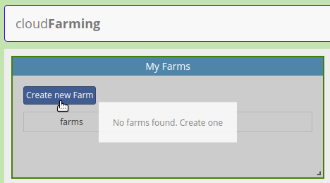
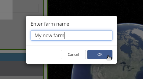
Go to the 'My Farms' pane and click the 'Create new Farm' button. You will be prompted to enter a name for your new Farm. Type the name and press OK.

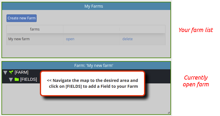
This pane, 'My Farms', will also show you the list of all the farms that you have created and you will be able to open or delete farms from it.

Below the 'My Farms' pane you will see the 'Farm' pane which will show you the structure of the newly created farm, or the one you have opened.

Each farm consists of one or more fields. Each field, in turn, can contain multiple exclusion areas and routes. This structure is represented in the 'Farm' pane with a tree view.

An overlay message will remind you that you haven't created any Fields on your new Farm yet and that should be the next step.

Adding fields to your farm

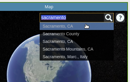
First of all you must navigate the map until you find the place where your farm will be. To do this, you can use the geocoder, a location search tool that flies the camera to a queried location. Click the magnifying glass icon at the top right of the 'Map' pane and type the location you are looking for.

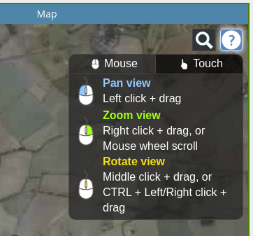
To display instructions for navigating the map with the mouse or on a touch device, click the question mark icon.

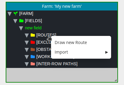
Once you have the location on the map, go to the 'Farm' pane and click on the [FIELDS] node of the tree view. The context menu will appear and you will find two options to add new fields: drawing it or importing a file.

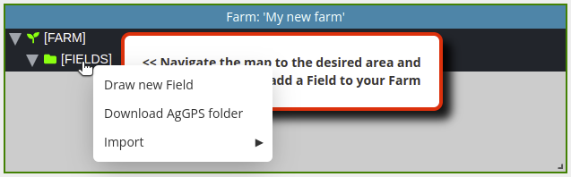
- Create Fields by drawing on the map:

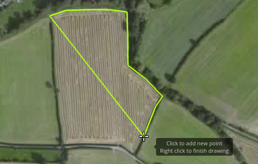
Click on the "Draw new Field" menu option and start to draw on the map by adding points with the mouse to define the field boundary with a polygon. Finish the boundary by right clicking; CloudFarming will ask for a name for the new field.

- Create Fields by importing a Shapefile:

Click the 'Import'->'Shapefile (.shp)' menu option and select only the .shp file, which must contain a 'Polygon' type shape.

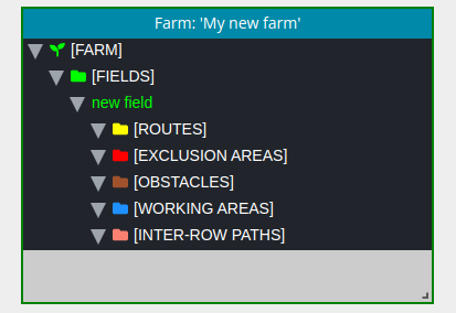
The new field is added under the [FIELDS] node in the tree view of the 'Farm' pane, and four subnodes are automatically created: [ROUTES], [EXCLUSION AREAS], [OBSTACLES], [WORKING_AREAS] and [INTER-ROW PATHS]. You can click these sub-nodes to add these entities to the field in a similar way to how you created the new field.

Adding exclusion areas to fields

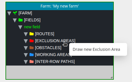
Go to the 'Farm' pane and click on the [EXCLUSION AREAS] node that is under the field to which you want to add an exclusion area. The context menu with the option 'Draw new Exclusion Area' enabled will appear. Click on it and start to draw the exclusion area inside the chosen field.

Add the points with the mouse on the map and finish by right-clicking. Enter the name for the new exclusion area. It will be added under the [EXCLUSION AREAS] node of the corresponding field.

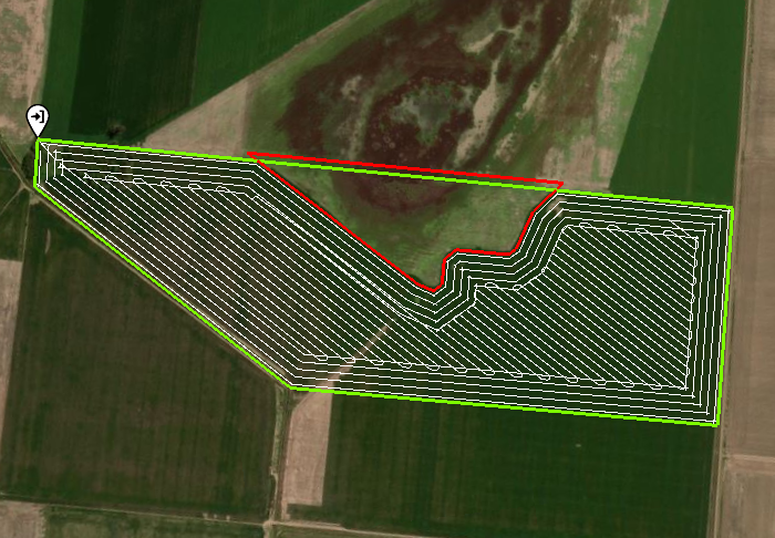
Exclusion areas are used only in the 'Open Field' version of the Route Planner, and they may exceed the field boundaries or be completely contained within the field.

In the first case, the Route Planner will simply calculate the new shape of the field, performing polygon clipping. In this way, the boundary of the field remains a simple polygon, and, if its shape allows it, the Route Planner could calculate a route without subdividing into subfields. The following figure shows such an example:

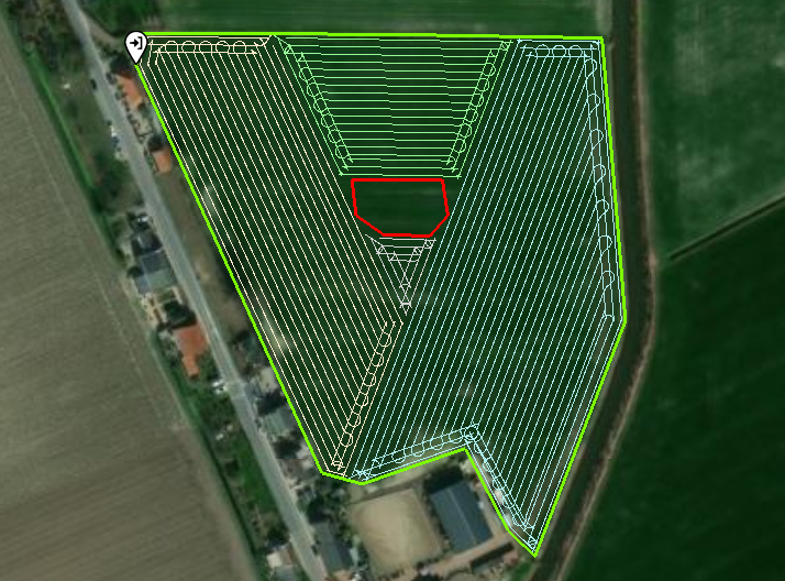
In the second case, when the exclusion area is contained within the field, the field is represented geometrically as a polygon with holes. In this situation, as shown in the following example, the field must necessarily be divided into subfields.

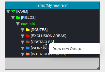
Adding obstacles to fields

Go to the 'Farm' pane and click on the [OBSTACLES] node that is under the field to which you want to add an obstacle. The context menu with the option 'Draw new Obstacle' enabled will appear. Click on it and start to draw the obstacle inside the chosen field.

Add the points with the mouse on the map and finish by right-clicking. Enter the name for the new obstacle. It will be added under the [OBSTACLES] node of the corresponding field.

Obstacles are also only used in the 'Open Field' version of Route Planner, and also represent sectors (in this case small, typically on the order of a few working widths) that will be excluded from the area to be worked. But unlike exclusion areas, obstacles do not require the Route Planner to divide into subfields. Instead, the vehicle deviates slightly from its original path to avoid them. The following image shows some examples:

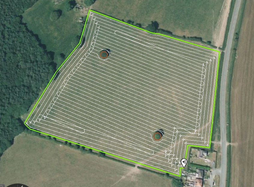
In the current version, only obstacles that are within the main field area (internal pattern with straight rows) are computed. The obstacles that are on the headland circuits require a more complex calculation and will be resolved in future versions.

Furthermore, the obstacles must be separated from each other, so that the vehicle must face a new obstacle only when it has finished avoiding the previous one.

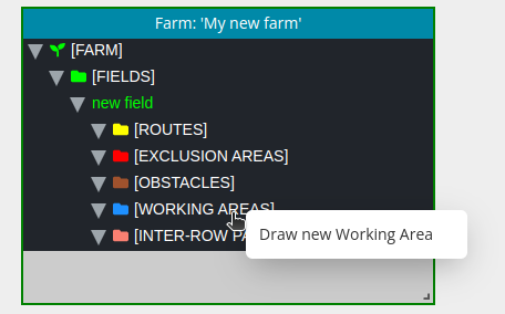
Adding working areas to fields

The working areas represent the region of the field that excludes headlands and can be useful for certain operations, such as intersecting a recorded route to remove the turns and replace them with turns generated by the Route Planner (see the 'Orchard' option in the Route Planner section).

You can add a working area by drawing on the map just like the rest of the entities.

Adding inter-row paths to fields

The inter-row paths are a collection of paths between the rows of an orchard that can be curves (polylines) and that the Route Planner can join with turns in order to generate a route.

There are two ways to add inter-rows paths to a field:

- Create Inter-row Paths by importing files:

Go to the treeview of the 'Farm' pane, and click on the [INTER-ROW PATHS] node under the corresponding Field. You will find the options to import the paths from a Shapefile or GeoJSON file. In the case of a Shapefile, you must select only the .shp file, which must only contain shapes of the type 'Polyline'. Equivalently, the GeoJSON file must contain only geometries of type 'LineString'.

The paths must be parallel or nearly parallel. The order does not matter and neither does it matter if some of them point in the opposite direction. CloudFarming will automatically sort them from one side to the other and make them all point in the same direction.

The imported rows will be shown as pink lines on the map.

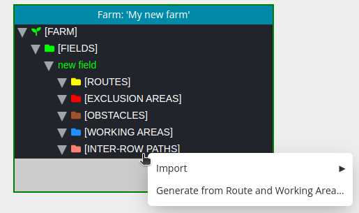
- Create Inter-row Paths by intersecting a Working Area and a Route:

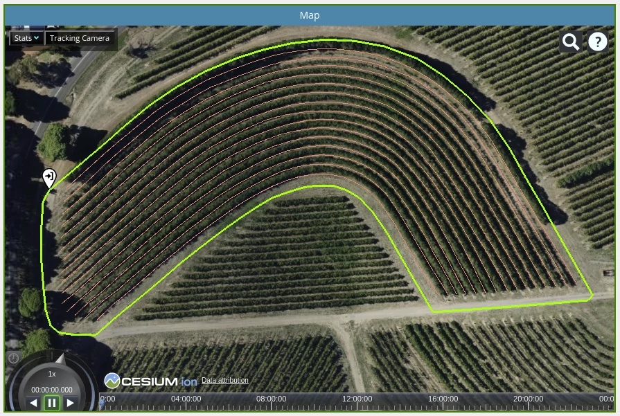
Go to the treeview of the 'Farm' pane, and click on the [INTER-ROW PATHS] node under the corresponding Field. Click the context menu option 'Generate from Route and Working Area...'. The window shown in the image below will appear and ask you to select the Route and Working Area to intersect.

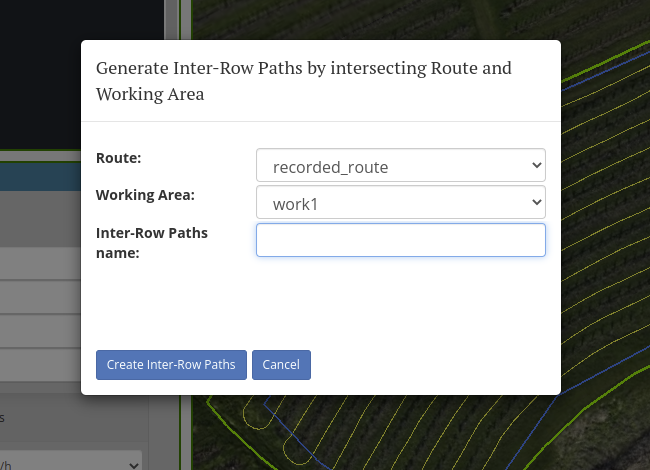
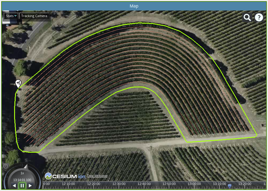
The route sections that are within the limits of the Working Area will be converted into a new collection of Inter-row paths. The following animated image shows the result of this process with an example:

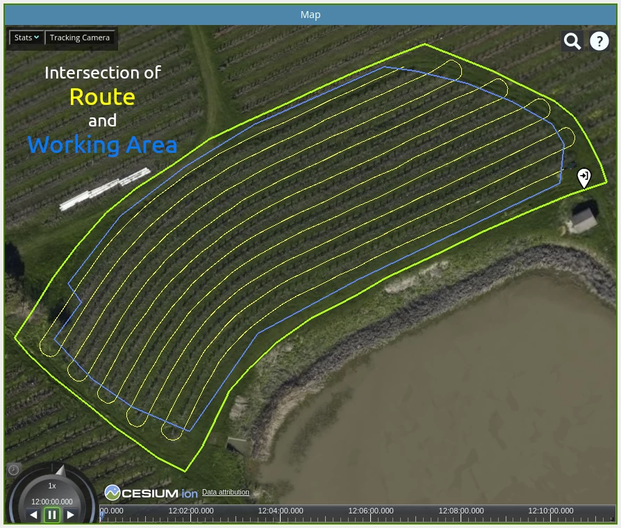
This technique allows you to record a driven route (or import a previously recorded one), intersect it with a Working Area to cut off the turns, and use the Route Planner ('Orchard' option) to replace them with new automatically generated turns.

Adding routes to a field

There are four ways to create routes in CloudFarming:

1 - Create Routes by drawing on the map:

Go to the 'Farm' pane and click on the [ROUTES] node that is under the field to which you want to add a route. The context menu will appear. Click the option 'Draw new Route' and start to draw the route inside the chosen field.

Add the waypoints with the mouse and finish by right-clicking. Enter the name for the new route. It will be added under the [ROUTES] node of the corresponding field.

2 - Create Routes by importing files:

Go to the 'Farm' pane, click on the [ROUTES] node that is under the field to which you want to add a route, select the the 'Import' option from the context menu and choose the file type (NMEA GPS log file or GeoJSON).

In case of choosing a GPS log file, it must be a text file with GPS data in NMEA format, containing at least GPGGA or GNGGA sentences, for example:

...
$GPRMC,135538.000,A,5629.3679,N,00935.3711,E,0.00,71.08,061009,,,A*5F
$GPGGA,135539.000,5629.3679,N,00935.3711,E,1,10,0.8,52.1,M,43.0,M,,0000*64
$GPGSA,A,3,29,25,21,31,30,10,05,13,16,06,,,1.5,0.8,1.3*35
$GPGSV,3,1,12,21,56,165,51,16,55,288,48,29,47,083,49,31,28,218,44*7A
$GPGSV,3,2,12,05,24,052,41,10,20,044,34,06,16,262,25,13,11,331,40*79
$GPGSV,3,3,12,25,09,336,25,30,07,136,38,03,04,266,,23,03,296,*74
...

When you choose to import the route from a GeoJSON file, CloudFarming will automatically detect and import any file that contains any of the following formats:

- Feature Collection containing a single LineString geometry
- Feature Collection containing multiple Point geometries
- Single Feature containing a single LineString
- Geometry Collection containing a single LineString
- Geometry Collection containing multiple Points
- Single Geometry containing a single LineString

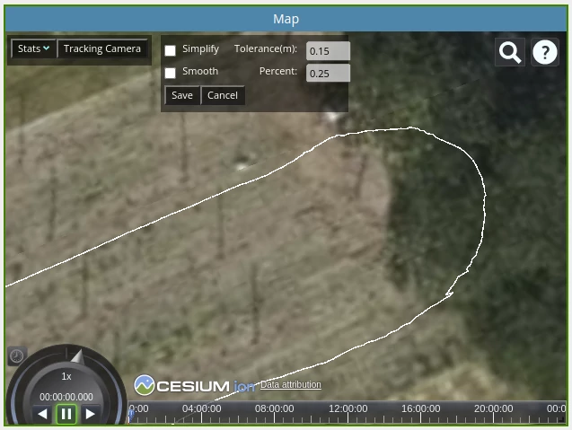
Once you select the file to import in the 'Open File' window, you will get a preview of the route drawn with a white line. At the same time, a dialog box will appear on the map that will optionally allow you to simplify and smooth the route. These techniques are particularly useful when importing routes that have been recorded from a vehicle equipped with a GPS device.

Simplify option: removes points from the original route, within a certain tolerance (expressed in meters).

Smooth option: it doubles the number of points of the route to make the curve smoother.

You can vary the value of the parameters and see how the preview of the route changes. Once you are satisfied with the result, click 'Save' to store the route.

The following animated image shows this process of importing, processing and saving the route.

3 - Create Routes by recording ROS messages:

In order to create a route this way, you must first connect CloudFarming to a ROS network, and subscribe to a topic of the type sensor_msgs/NavSatFix. You can see the details on how to do this in the 'CloudFarming and ROS' section

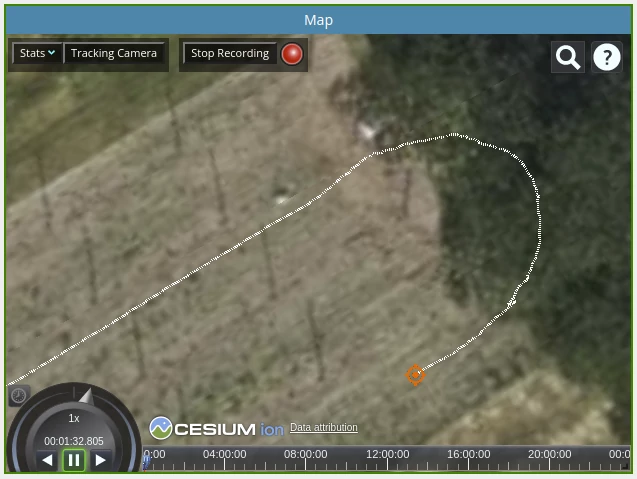
As soon as CloudFarming receives the first NavSatFix message, the GPS icon will be positioned at the coordinates obteined, and the 'Start/Stop Recording' button will be displayed at the top of the map.

When the icon is at the position from where you want to start recording the route, click "Start recording". A dashed white path will begin to be drawn (and the simulated LED will start blinking to remind you that you are recording a route)

When you want to stop recording, click the button again. From there, the process is exactly the same as when you import a route: you will see a preview of the route and a box to simplify and smooth the original route (see the previous point -Create Routes by importing files- for more details). When you are satisfied with the preview, click 'Save' and a window will be displayed with the options to save the recorded route (name and field to which it belongs). You can also choose to discard the route recorded up to that point.

The following animated image shows how to record, process and save the route.

4 - Create Routes by using the Route Planner:

The Route Planner is a fundamental part of CloudFarming, and therefore its use is described in detail in the next section.

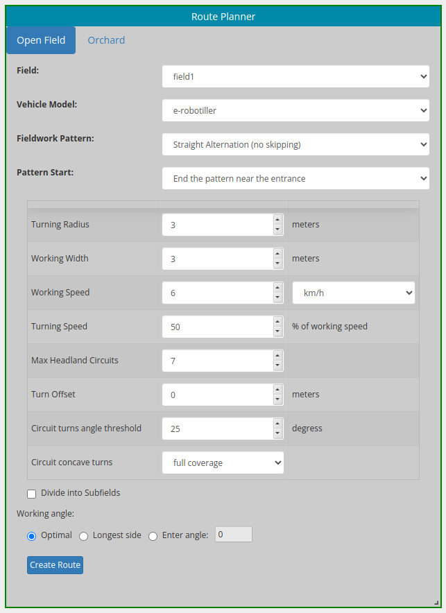
Using the Route Planner

This is one of the most important components of CloudFarming. The Route Planner calculates the optimal route for a field based on its geometry and multiple parameters defined by the user.

The Route Planner pane presents two tabs that correspond to different versions according to the type of planning you are looking for:

1. 'Open Field'
2. 'Orchard'

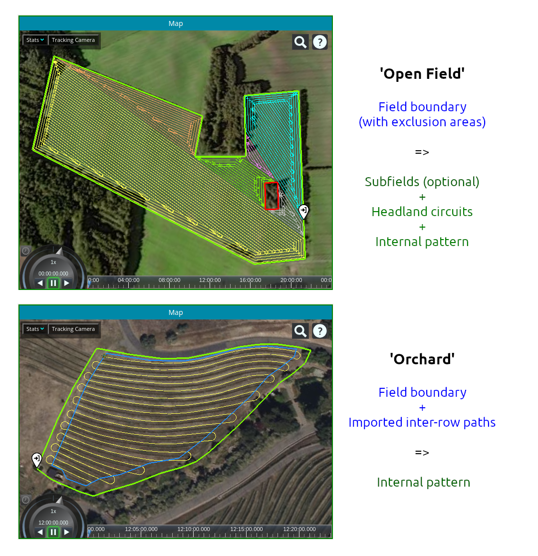
1 - Open Field

The generated route is made up of two parts:

- Headland circuits: following the contour of the field boundary
- Internal pattern: parallel straight rows for the main field

The field can be divided into subfields (optionally in some cases, mandatory in others, depending on its geometry). In the case of splitting, this pattern (headland circuits + internal rows) will be applied to each subfield.

The parameters that the user must configure are:

Field: the field for which you want to calculate the route.

Vehicle Model: 3D model that will be used in the 3D animation. Models of 'Robotiller' (https://www.e-robotiller.nl/) and eTrac (https://www.farmertronics.com/) projects are currently available.

Fieldwork pattern: for the main field area.
The options are:
- Straight Alternation (no skipping). The vehicle traverses the main field with a back and forth pattern of adjacent rows.
- Skip and Fill Pattern (SFP). The route skips rows. The number of rows skipped N can be 3, 5, or 7. The vehicle skips N rows forward on one side, and N-2 backward on the opposite side. At the beginning and at the end of the route, it performs 1 row skips to be able to complete all the rows.

(See the comparison between the different types of fieldwork patterns in an orchard in the 'Statistics' section)

Pattern Start: the available options are "End the pattern near the entrance" and "Start the pattern near the entrance". Determines whether the internal pattern will start or end near the field entrance

Turning Radius: of the vehicle that will use the route.

Working Width: distance between adjacent rows.

Working Speed: of the vehicle.

Headland Circuits: the number of headland circuits. When the system does not find enough space to make all the circuits, the number will be automatically reduced.

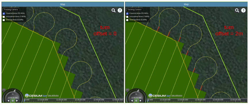
Turn offset: a straight path is added before and after making the turn. This gives a margin to align the vehicle before entering the work zone, and to keep it aligned before leaving it completely. The following image graphically shows the effect of setting a turn offset value.

Circuit turns angle threshold: establishes a threshold angle from which the turning maneuver will be implemented in the headland circuits. It affects both concave and convex turns. In the example in the following video, on the left a value of 0º has been used for the parameter and on the right 30º. The first two turns have values of approximately 90 and 45º, therefore there is no difference. The last turn is less than 30º, therefore in the right version the turning maneuver (convex in this case) is not performed.

Circuit concave turns: defines how concave turns will be made in headland circuits. If the option "full coverage" is selected, the turning maneuver includes two reverse movements. If the option is 'simple', only one reverse movement is performed. The following video shows the difference. On the left, the 'full coverage' version. As you can see at the end of the video, the turn requires more time, but full coverage of the treated area is achieved.

Working Angle: angle that determines the direction of the rows in the internal pattern. This parameter will be used when the field is not divided into subfields. If you choose the "subdivide" option, it will be ignored.

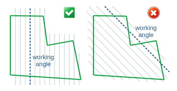
In order for the "open field" pattern (headland circuits + internal rows) to be applied to the entire field (without subdivision), the following conditions must be met:
1 - The field must not have exclusion areas
2 - The polygon that defines the field boundary must be monotone with respect to the working angle. That is, any line whose direction is given by the working angle must intersect the field boundary polygon only at two points, as shown in the following figure.

The options to establish the working angle are the following:
1 - "Optimal": The route planner will look for the working angle that generates the smallest number of headland turns
2 - "Longest side": will choose the angle of the longest side of the field boundary polygon
3 - "Enter angle": allows you to type a specific value in degrees for the working angle (0º = horizontal line, west-east axis, positive counterclockwise)

Divide into Subfields: When this option is not activated the field will not be subdivided and the working angle will be determined by the parameter described above. The parameters that follow below will be ignored.

When enabled, the field will be divided into subfields. The 'workingAngle' parameter will be ignored and the system will assign each subfield its own working angle. The subdivision will be carried out according to the following parameters:

Area Cost Coefficient and Time Cost Coefficient: these parameters are used in the cost function that selects the best subregion. When the ACC is increased compared to the TCC, the Route Planner algorithm will tend to choose subregions that have the largest possible area, regardless of the time it takes for the tractor to complete the route. When the TCC is increased compared to the other, sub-regions are sought that try to minimize the time (usually, routes with fewer turns).

Threshold Right Angle and Threshold Collinear Angle: used internally by the Route Planner algorithm to determine the shape of the subregions generated. The lower the values, the greater the number of subregions will tend to be.

2 - Orchard

Unlike the type 'Open Field', in the case of orchards the route must be generated following the constraint of existing tree rows.

Therefore, to use this option, the Field must have at least one set of 'Inter-row Paths' (see details in the 'Adding Inter-row Paths' section).

The route planner will generate the complete route by joining these inter-row paths with turns. You can change the fieldwork pattern to try different sequences in which the paths will be traversed. The selected pattern, together with the turning radius, will determine the turns generated.

The rest of the parameters are similar to the 'Open Field' option.

The animated image below shows an example of a route created by the route planner from the inter-row paths.

3D animation

When you use the 'Open Field' or 'Orchard' options, after generating a route, a 3D model of the vehicle is automatically created at the entrance point of the field.

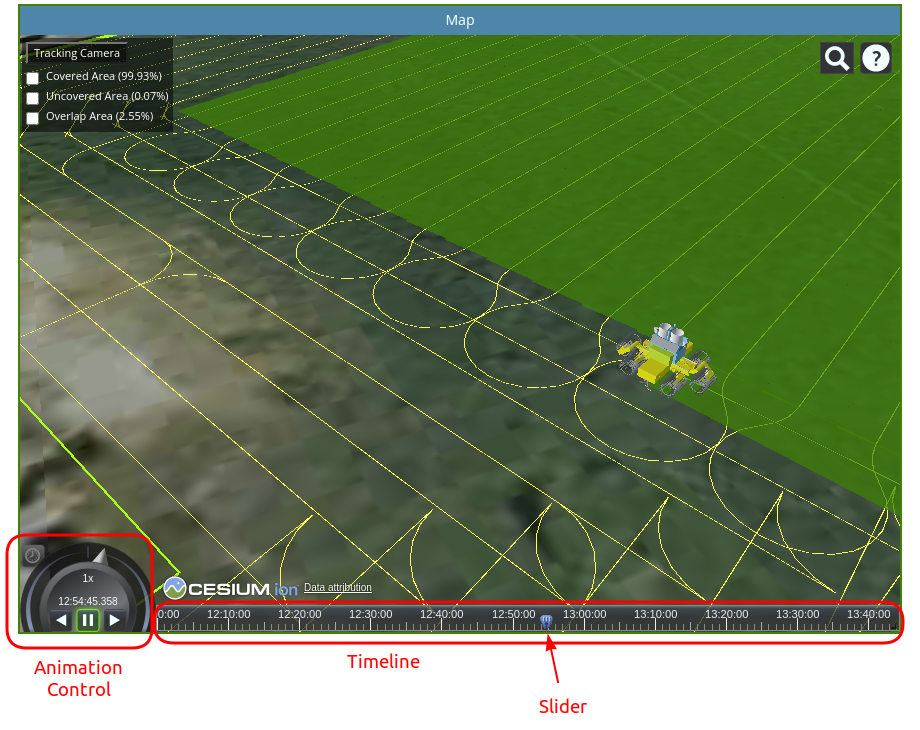
Then, you can go to the Animation Control and click the 'Play Forward' button to start the route simulation. This tool allows to analyze the vehicle's path through the planned route. The progress of the worked area is shown as the vehicle moves.

You can adjust the clock multiplier to speed up the animation or drag the timeline slider to go to any time in the animation.

Click the 'Tracking Camera' button to enable the camera that follows the vehicle.

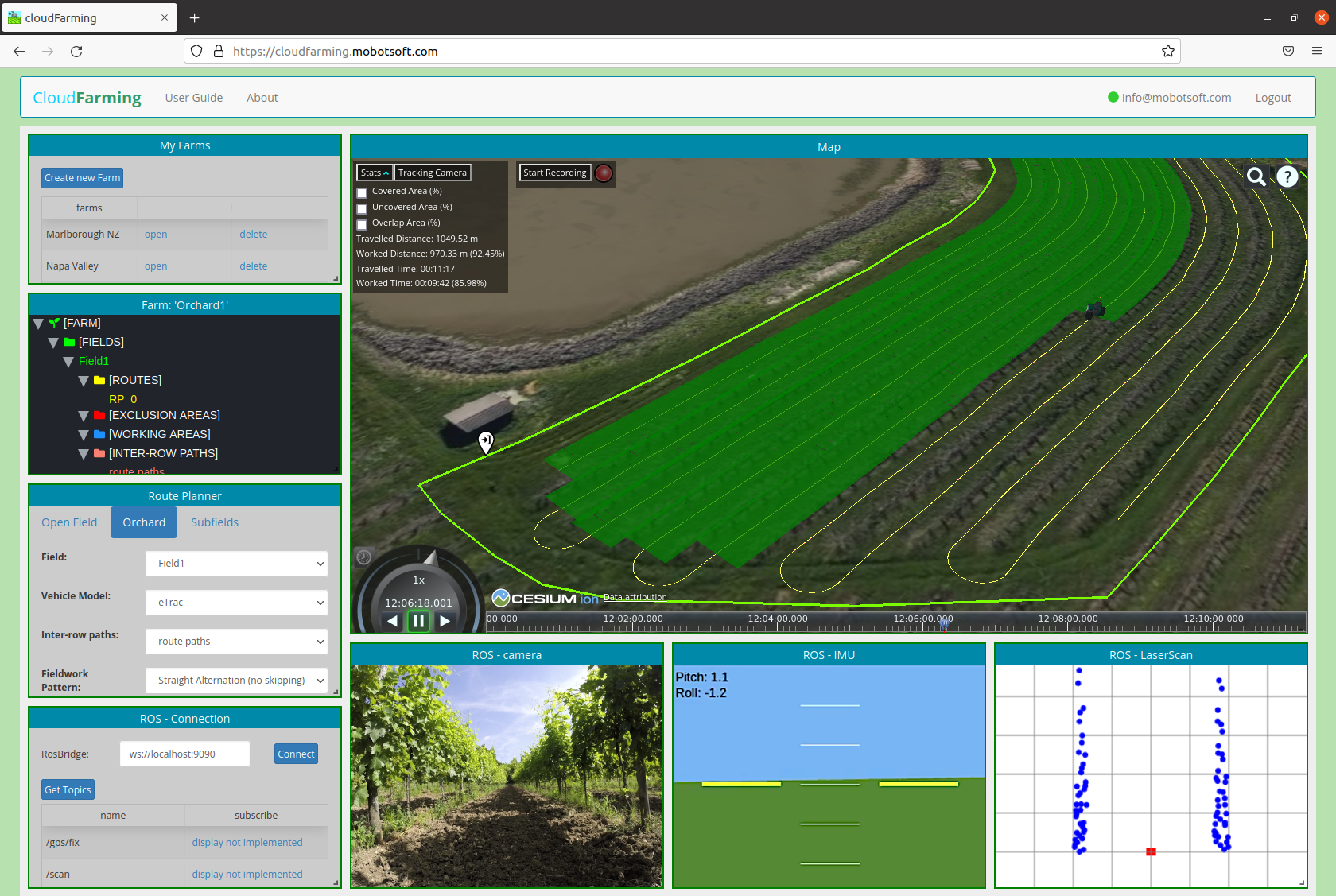
Statistics

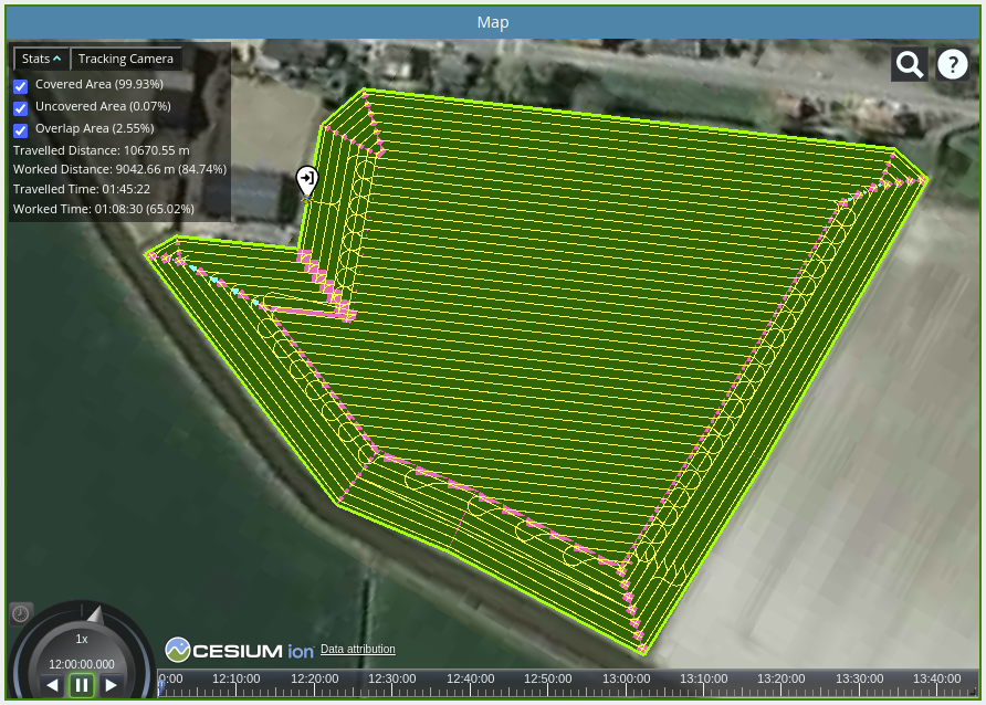
When a route is calculated with the Route Planner, the covered, overlap and uncovered areas are automatically calculated, as well as their corresponding percentages relative to the total area.

Click on the statistics checkboxes to show or hide these areas on the map.

In addition, the Travelled Distance values and the Worked/Traveled distance ratio are calculated, and the same with Travelled and Worked Time.

This allows you to compare the results achieved with different types of fieldwork patterns and find the optimal one. For example, the following image shows the routes generated in an orchard using different patterns.

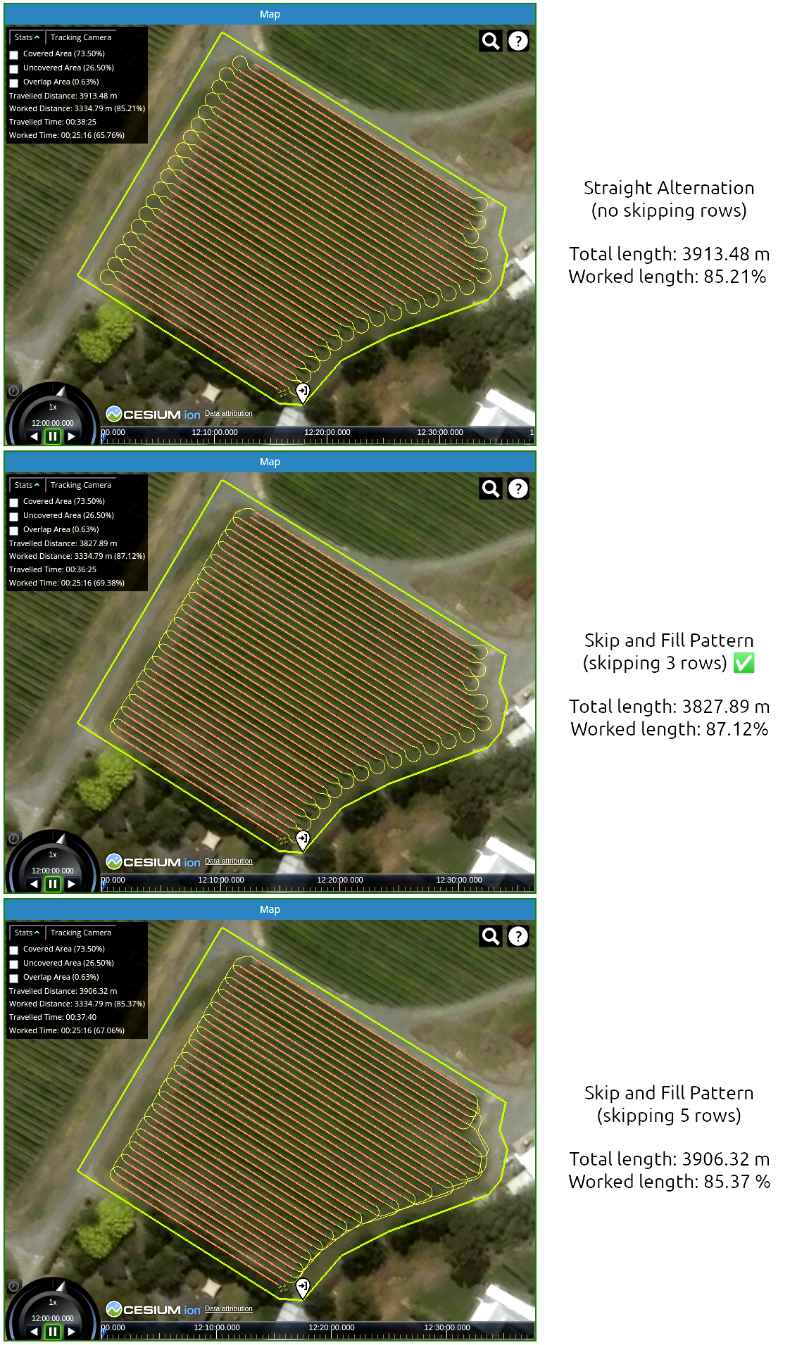
In the first case, the "Straight Alternation (no skipping)" pattern was used. The turning radius of the vehicle requires "bulb" type headland turns, resulting in a total distance traveled of 3913.48 m and 85.21% of it is worked.

In the second case, the "Skip and Fill Pattern (SFP)" skipping 3 rows was used. This pattern generates bulb turns on one side of the orchard, and (more efficient in this case) long turns on the opposite side. In this way, a total length of 3827.89 m is obtained, less than in the previous case, and also a better working distance ratio, 87.12%.

In the third case, the "Skip and Fill Pattern (SFP)" skipping 5 rows was selected. In this case, long turns are obtained on both sides of the orchard, but on one side they are too long and the numbers get worse again (total distance: 3906.32 m, worked distance: 85.37%), resulting in the second option (SFP - 3 rows) as the most efficient.

CloudFarming and ROS

CloudFarming connects to ROS (Robot Operating System) to send and receive messages in a local network through Rosbridge.

This tutorial will show you how to install and run Rosbridge:
https://wiki.ros.org/rosbridge_suite/Tutorials/RunningRosbridge

Connection

Once you have Rosbridge running on your local network, go to the 'ROS-Connection' pane of CloudFarming. Enter the URL where Rosbridge is running. In this example, CloudFarming will connect to Rosbridge on localhost using the default port 9090:

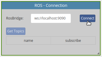
Click the 'Connect' button to establish the connection.

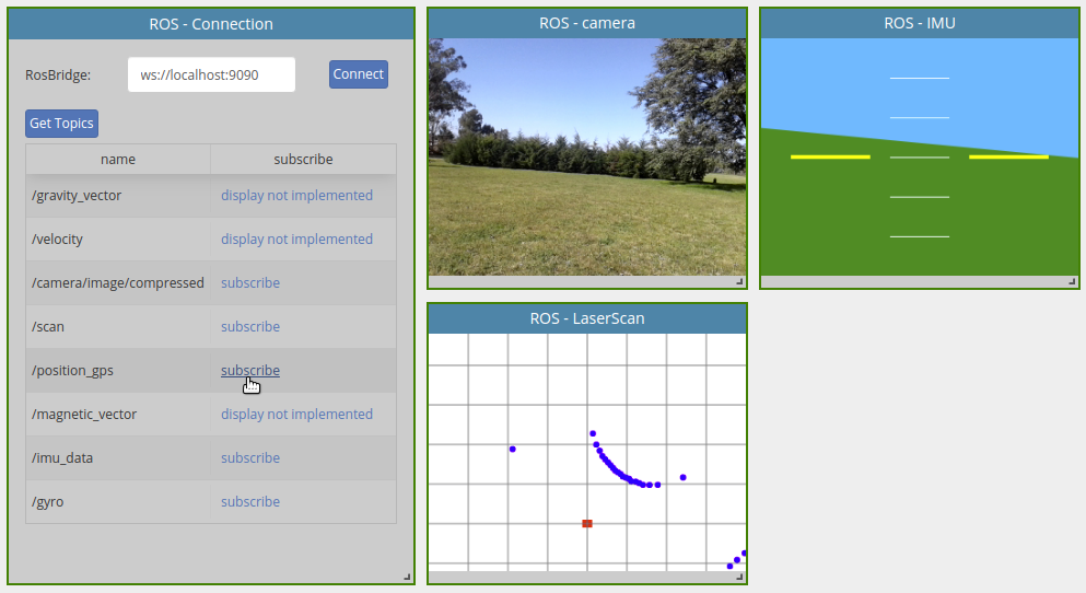
Getting topic list

If the connection is successful, the button 'Get Topics' will be enabled. Click it to obtain the list of active topics in ROS. You have the option to subscribe to those topics that have a built-in display implemented in CloudFarming. For the time being, displays for types 'sensor_msgs/CompressedImage', 'sensor_msgs/Imu' and 'sensor_msgs/LaserScan' were implemented.

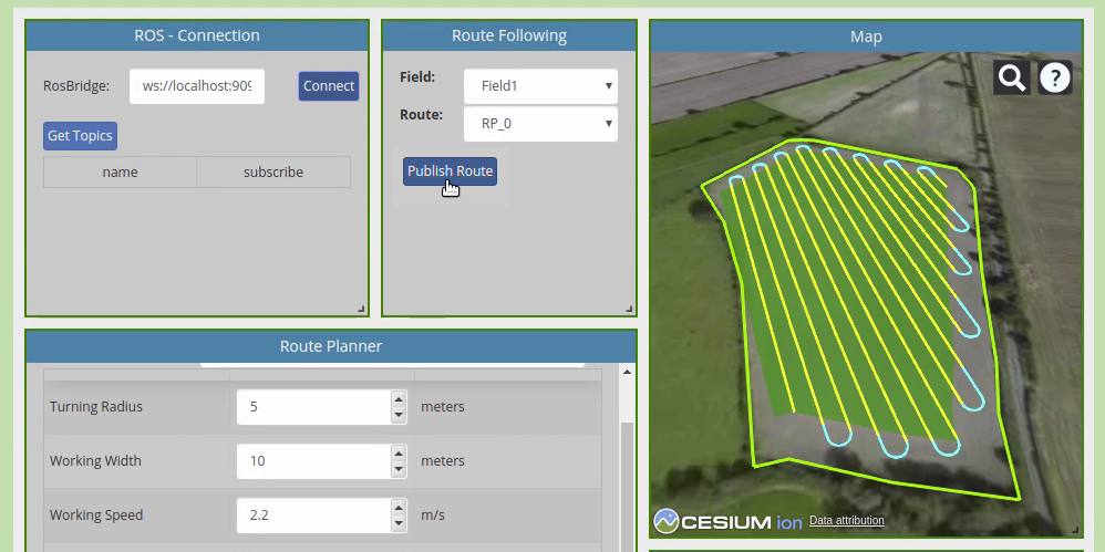
Publishing Routes

CloudFarming can also publish messages on the ROS network. You can for example publish a route. To do this, go to the 'Route Following' pane, select the field and route, and click the 'Publish Route' button.

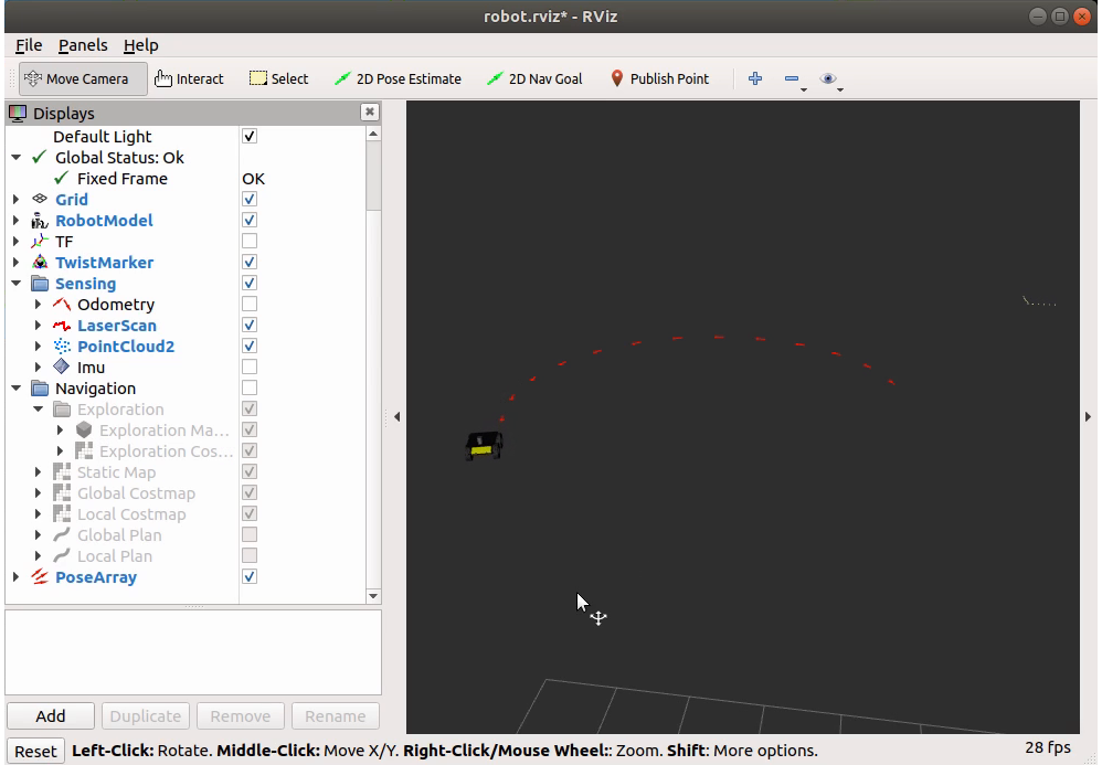
A message of type 'geometry_msgs/PoseArray' with name '/route' and UTM coordinates will be published.

In the example below, you can see in RViz how a ROS package receives the route and executes a waypoint navigation algorithm to control a simulated Husky UGV.